BIO 349L, Project 3: Analysis of a priori data
First, we’ll read the data from the Google Sheet from
where it is hosted. We’ll save the data as 2015.csv and 2016.csv in a Data/
sub-directory:
gs_title("Module3") %>%
  gs_read_csv("2015") %>%
  group_by(Time, MolarityNaF) %>%
  mutate(Total = Arms0 + Arms1 + Arms2) %>%
  export("Data/2015.csv")

gs_title("Module3") %>%
  gs_read_csv("2016") %>%
  group_by(Treatment, Time) %>%
  mutate(Total = Arms0 + Arms1 + Arms2) %>%
  export("Data/2016.csv")
Then, we read the data in as a data.frame:
df_15 <- readr::read_csv("~/Github/BIO349L/Module03/Data/2015.csv")
df_16 <- readr::read_csv("~/Github/BIO349L/Module03/Data/2016.csv")
Variables
Dependent Variables
These datasets contains 837 observations from 2016 and 5,467 observations from 2015.
These datasets focus on the development of sea urchin embryos that were exposed to sodium fluoride (NaF) during development. In the 2015 set, both the concentration of NaF and the duration of exposure were varied. The total number of observations for both these variables can been seen in the table output below:
| NaF | 2-24 h | 2-48 h | 24-48 h | Control |
|---|---|---|---|---|
| 0.000 | NA | NA | NA | 3019 |
| 0.002 | 341 | 440 | 354 | NA |
| 0.004 | 438 | 446 | 429 | NA |
In the 2016 set, the concentration of NaF was further simplified to a binary
variable (either control or NaF), and more nuanced time intervals were examined.
These time intervals are illustrated in the plot below:
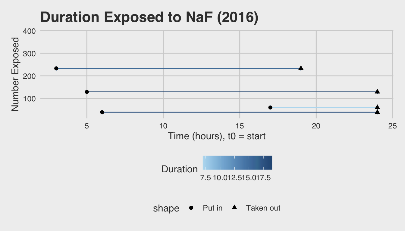
Note: Because the control embryos weren’t exposed, and thus had no interval of exposure, they’ve been omitted from the above plot (n= 376).
Independent Variables
The variable being observed in both these datasets is the number of “arms” that developed. Under normal developmental circumstances embryos develop two arms, but exposure to NaF is believed to reduce the number of arms that develop.
For each group, the number of embryos with 0, 1, and 2 arms were counted and the total recorded.
Results
Results: Concentration of NaF
Plot1 <- readr::read_csv("~/Github/BIO349L/Module03/Data/2015.csv") %>%
  ggplot(aes(x=Arms2/Total, fill=factor(MolarityNaF),
             color=factor(MolarityNaF))) +
  geom_density(alpha=0.5) +
  labs(x="Had Two Arms") +
  scale_fill_brewer(name="Molarity of NaF", palette = 4) +
  scale_color_brewer(name="Molarity of NaF", palette = 2, type = "qual") +
  scale_x_continuous(labels = percent) +
theme_fivethirtyeight() + theme(axis.title=element_text())## Parsed with column specification:
## cols(
## Time = col_character(),
## MolarityNaF = col_double(),
## Treatment = col_character(),
## Group = col_character(),
## Arms0 = col_double(),
## Arms1 = col_double(),
## Arms2 = col_double(),
## Total = col_double()
## )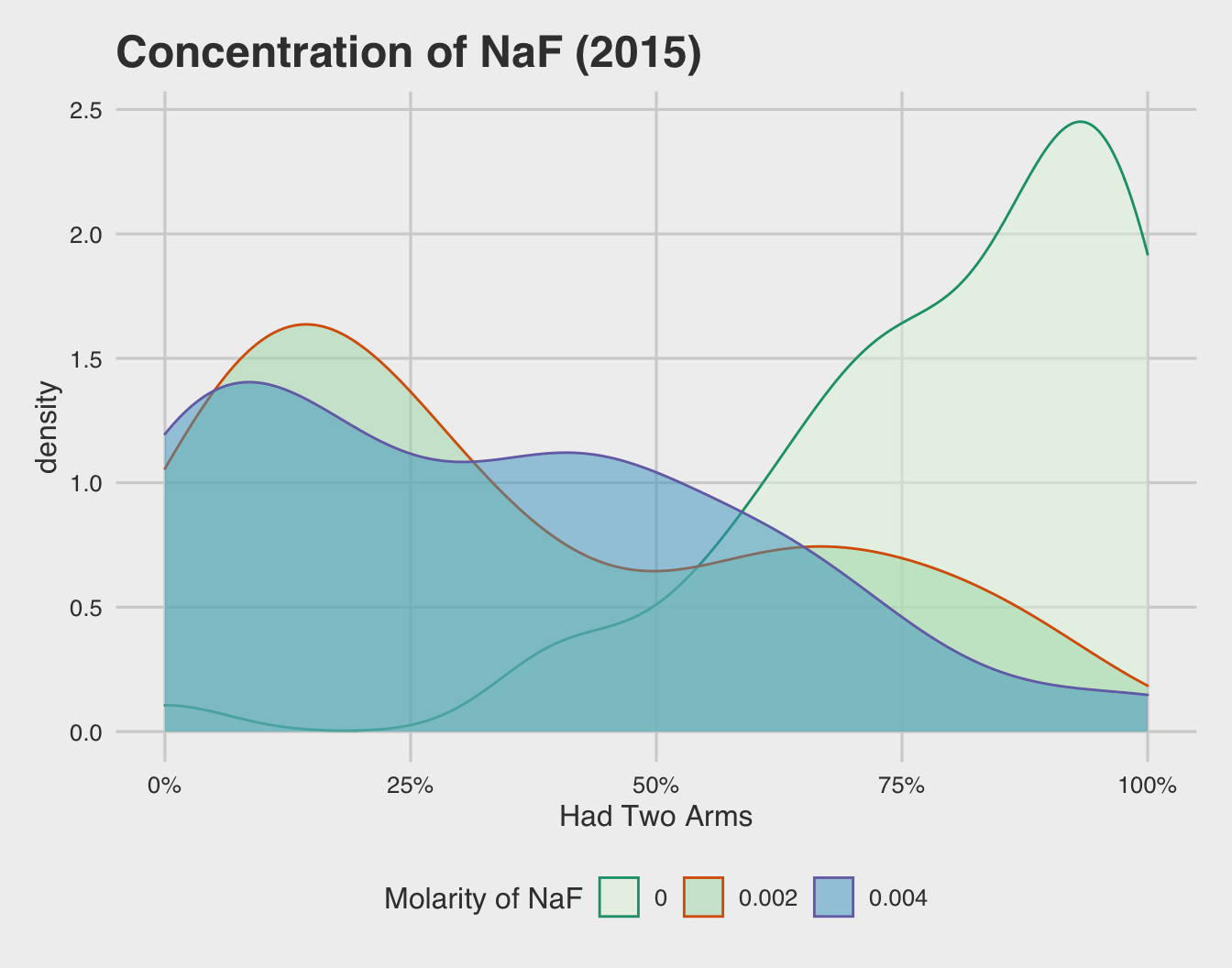
Above is a density plot illustrating the percentage of embryos who developed both arms, with each density curve colored by the concentration of NaF embryos were exposed to during development. It’s evidently clear that no exposure to NaF (the lightest blue) has a severe rightward skew. This skew indicates that the vast majority of embryos in the control group developed normally.
Unsurprisingly, the embryos exposed to NaF had a leftward skew, indicating a good number of embryos didn’t develop to have two arms. More importantly, it appears that both levels of NaF exposure (2 mM and 4 mM) have similar density distributions. This indicates that the level of exposure isn’t nearly as important as wither or not embryos are exposed in the first place.
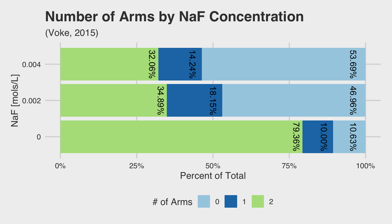
This same observation can be seen if we examine the within-group distribution for each NaF concentration. The bar plot below shows the relative percentage of embryos with 0, 1, or 2 arms for each treatment group. The percentages are nearly identical for both concentrations, but show a marked difference from the control group (represented by 0 mols/L of NaF).
df_15 %>%
  group_by(NaF=MolarityNaF, Treatment) %>%
  summarise(
    Total = sum(Total),
    Arms0 = sum(Arms0)/Total,
    Arms1 = sum(Arms1)/Total,
    Arms2 = sum(Arms2)/Total) %>%
  gather(Arms, Percent, Arms0:Arms2) %>%
  mutate(
    Arms = stringr::str_replace(Arms, "Arms", ""),
    Arms = paste(Arms, "Arms"),
    Percent = percent(Percent)) %>%
  spread(Arms, Percent) %>%
  select(-Treatment, -Total) %>%
knitr::kable()| NaF | 0 Arms | 1 Arms | 2 Arms |
|---|---|---|---|
| 0.000 | 10.63% | 10.00% | 79.36% |
| 0.002 | 47% | 18% | 35% |
| 0.004 | 54% | 14% | 32% |
Results: Onset & Duration of Exposure
Given that the concentration of NaF doesn’t seem to be that important, the next logical question becomes about the timing of exposure. To explore this in more detail, we’ll take the same density plot that we discussed above, and facet it by each time interval of exposure:
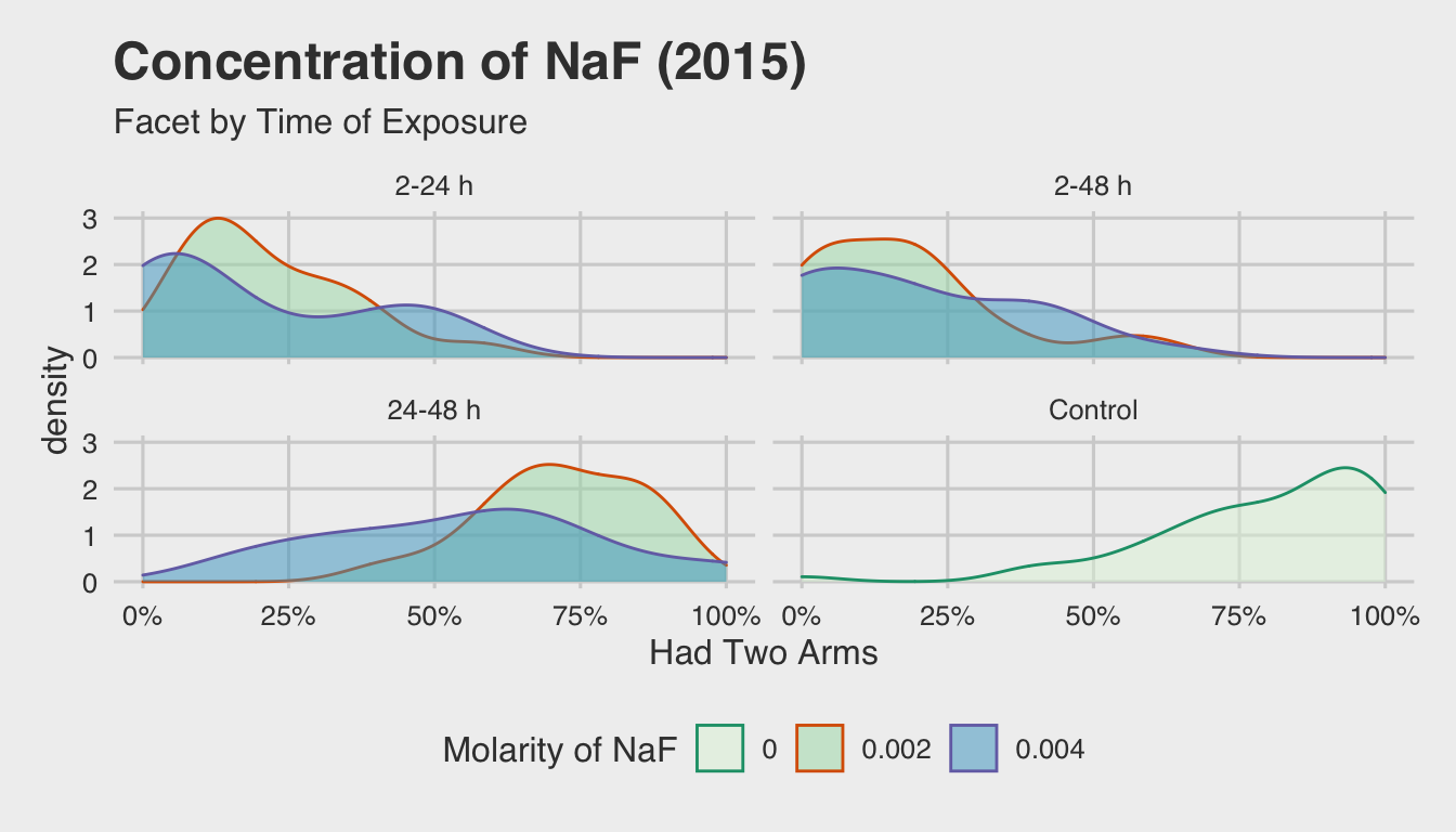
This illustrates the effects of early exposure in determining the number of arms
that eventually form. In the top two facets (2-24 h and 2-48 h) show a marked
decrease in the percentage of normal embryos that develop, as indicated by the
leftward skew. On the other hand, embryos that were exposed after 24 h or not
exposed at all (i.e. the NA facet) display a rightward skew.
From this we can conclude that early exposure is a key component in disrupting arm development. Likewise, we see that these new density distributions hold true to our findings regarding the insignificance of the concentration of NaF.
Again, this can also be illustrated using bar plots:
## Warning: `data_frame()` is deprecated as of tibble 1.1.0.
## Please use `tibble()` instead.
## This warning is displayed once every 8 hours.
## Call `lifecycle::last_warnings()` to see where this warning was generated.
## Joining, by = "Time"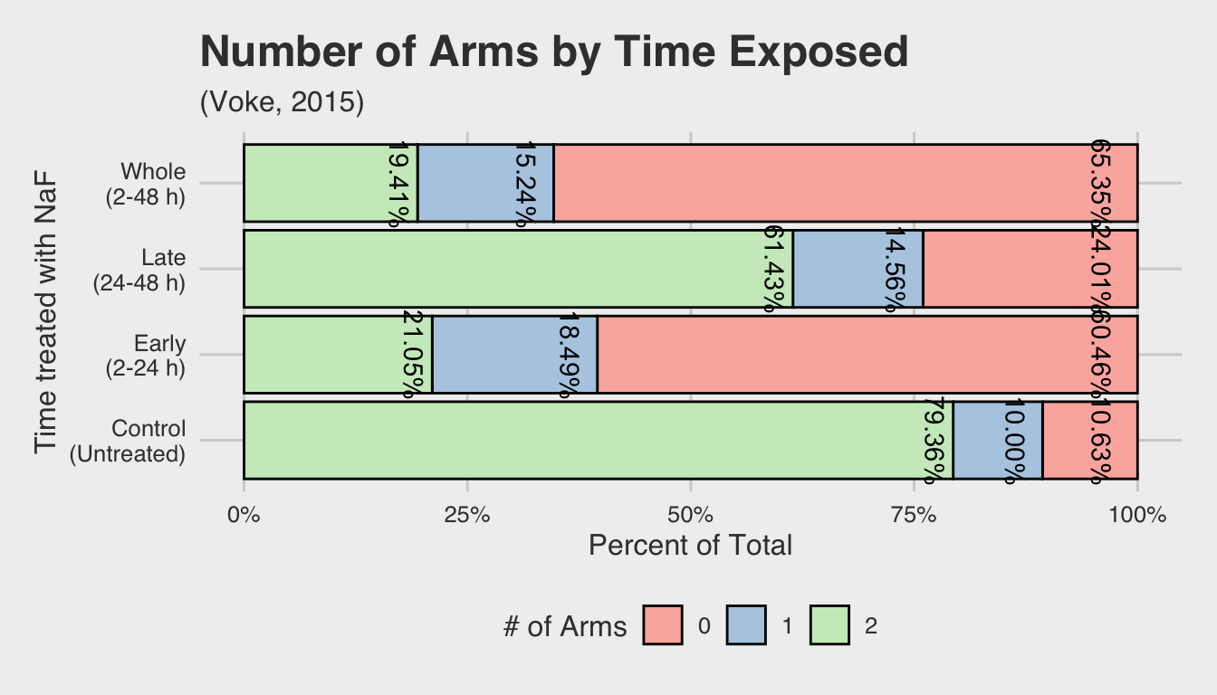
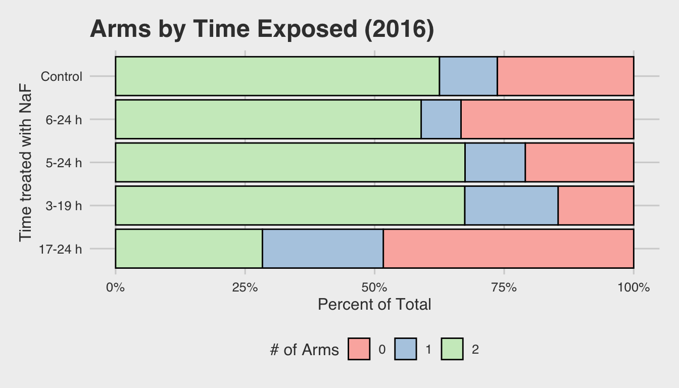
Next, we’ll take a look at the 2016 data. As mentioned above, this dataset takes a deeper look into the timing of exposure in the first 24 hours of development.
--- LICENSE ---

Copyright (C) 2016 Hunter Ratliff

This program is free software: you can redistribute it and/or modify
it under the terms of the GNU General Public License as published by
the Free Software Foundation, either version 3 of the License, or
(at your option) any later version.

This program is distributed in the hope that it will be useful,
but WITHOUT ANY WARRANTY; without even the implied warranty of
MERCHANTABILITY or FITNESS FOR A PARTICULAR PURPOSE.  See the
GNU General Public License for more details.

You should have received a copy of the GNU General Public License
along with this program.  If not, see <http://www.gnu.org/licenses/>.
This is an R Markdown document. Markdown is a simple formatting syntax for authoring HTML, PDF, and MS Word documents. For more details on using R Markdown see http://rmarkdown.rstudio.com.
In the spirit of Reproducible Research, below is the information About the R Session at the time it was compiled1:
devtools::package_info()
##  package      * version date       lib source
##  assertthat     0.2.1   2019-03-21 [1] CRAN (R 3.6.0)
##  backports      1.1.6   2020-04-05 [1] CRAN (R 3.6.2)
##  blogdown       0.18    2020-03-04 [1] CRAN (R 3.6.0)
##  bookdown       0.18    2020-03-05 [1] CRAN (R 3.6.0)
##  callr          3.4.3   2020-03-28 [1] CRAN (R 3.6.2)
##  cellranger     1.1.0   2016-07-27 [1] CRAN (R 3.6.0)
##  cli            2.0.2   2020-02-28 [1] CRAN (R 3.6.0)
##  colorspace     1.4-1   2019-03-18 [1] CRAN (R 3.6.0)
##  crayon         1.3.4   2017-09-16 [1] CRAN (R 3.6.0)
##  curl           4.3     2019-12-02 [1] CRAN (R 3.6.0)
##  data.table     1.12.8  2019-12-09 [1] CRAN (R 3.6.0)
##  desc           1.2.0   2018-05-01 [1] CRAN (R 3.6.0)
##  devtools       2.2.2   2020-02-17 [1] CRAN (R 3.6.0)
##  digest         0.6.25  2020-02-23 [1] CRAN (R 3.6.0)
##  dplyr        * 0.8.5   2020-03-07 [1] CRAN (R 3.6.0)
##  ellipsis       0.3.0   2019-09-20 [1] CRAN (R 3.6.0)
##  evaluate       0.14    2019-05-28 [1] CRAN (R 3.6.0)
##  fansi          0.4.1   2020-01-08 [1] CRAN (R 3.6.0)
##  farver         2.0.3   2020-01-16 [1] CRAN (R 3.6.0)
##  forcats        0.5.0   2020-03-01 [1] CRAN (R 3.6.0)
##  foreign        0.8-75  2020-01-20 [1] CRAN (R 3.6.3)
##  fs             1.4.1   2020-04-04 [1] CRAN (R 3.6.2)
##  ggplot2      * 3.3.0   2020-03-05 [1] CRAN (R 3.6.0)
##  ggthemes     * 4.2.0   2019-05-13 [1] CRAN (R 3.6.0)
##  glue           1.4.0   2020-04-03 [1] CRAN (R 3.6.2)
##  gtable         0.3.0   2019-03-25 [1] CRAN (R 3.6.0)
##  haven          2.2.0   2019-11-08 [1] CRAN (R 3.6.0)
##  highr          0.8     2019-03-20 [1] CRAN (R 3.6.0)
##  hms            0.5.3   2020-01-08 [1] CRAN (R 3.6.0)
##  htmltools      0.4.0   2019-10-04 [1] CRAN (R 3.6.0)
##  knitr          1.28    2020-02-06 [1] CRAN (R 3.6.0)
##  labeling       0.3     2014-08-23 [1] CRAN (R 3.6.0)
##  lifecycle      0.2.0   2020-03-06 [1] CRAN (R 3.6.0)
##  magrittr       1.5     2014-11-22 [1] CRAN (R 3.6.0)
##  memoise        1.1.0   2017-04-21 [1] CRAN (R 3.6.0)
##  munsell        0.5.0   2018-06-12 [1] CRAN (R 3.6.0)
##  openxlsx       4.1.4   2019-12-06 [1] CRAN (R 3.6.0)
##  pillar         1.4.3   2019-12-20 [1] CRAN (R 3.6.0)
##  pkgbuild       1.0.6   2019-10-09 [1] CRAN (R 3.6.0)
##  pkgconfig      2.0.3   2019-09-22 [1] CRAN (R 3.6.0)
##  pkgload        1.0.2   2018-10-29 [1] CRAN (R 3.6.0)
##  prettyunits    1.1.1   2020-01-24 [1] CRAN (R 3.6.0)
##  processx       3.4.2   2020-02-09 [1] CRAN (R 3.6.0)
##  ps             1.3.2   2020-02-13 [1] CRAN (R 3.6.0)
##  purrr          0.3.4   2020-04-17 [1] CRAN (R 3.6.2)
##  R6             2.4.1   2019-11-12 [1] CRAN (R 3.6.0)
##  RColorBrewer   1.1-2   2014-12-07 [1] CRAN (R 3.6.0)
##  Rcpp           1.0.4.6 2020-04-09 [1] CRAN (R 3.6.3)
##  readr          1.3.1   2018-12-21 [1] CRAN (R 3.6.0)
##  readxl         1.3.1   2019-03-13 [1] CRAN (R 3.6.0)
##  remotes        2.1.1   2020-02-15 [1] CRAN (R 3.6.0)
##  rio          * 0.5.16  2018-11-26 [1] CRAN (R 3.6.0)
##  rlang          0.4.6   2020-05-02 [1] CRAN (R 3.6.2)
##  rmarkdown      2.1     2020-01-20 [1] CRAN (R 3.6.0)
##  rprojroot      1.3-2   2018-01-03 [1] CRAN (R 3.6.0)
##  scales       * 1.1.0   2019-11-18 [1] CRAN (R 3.6.0)
##  sessioninfo    1.1.1   2018-11-05 [1] CRAN (R 3.6.0)
##  stringi        1.4.6   2020-02-17 [1] CRAN (R 3.6.0)
##  stringr        1.4.0   2019-02-10 [1] CRAN (R 3.6.0)
##  testthat       2.3.2   2020-03-02 [1] CRAN (R 3.6.0)
##  tibble         3.0.0   2020-03-30 [1] CRAN (R 3.6.2)
##  tidyr        * 1.1.0   2020-05-20 [1] CRAN (R 3.6.2)
##  tidyselect     1.1.0   2020-05-11 [1] CRAN (R 3.6.2)
##  usethis        1.5.1   2019-07-04 [1] CRAN (R 3.6.0)
##  vctrs          0.3.0   2020-05-11 [1] CRAN (R 3.6.2)
##  withr          2.1.2   2018-03-15 [1] CRAN (R 3.6.0)
##  xfun           0.13    2020-04-13 [1] CRAN (R 3.6.3)
##  yaml           2.2.1   2020-02-01 [1] CRAN (R 3.6.0)
##  zip            2.0.4   2019-09-01 [1] CRAN (R 3.6.0)
##
## [1] /Library/Frameworks/R.framework/Versions/3.6/Resources/library
The date compiled may differ from the date the code was written because it get’s re-run when it’s uploaded to the site↩