Stats for the Healthy Relationship Text Campaign
The output below is for the analysis of the Healthy Relationship Text Campaign (HRTC) through UTMB’s Behavioral Health And Research (BHAR) office.
Source data can be requested from the Behavioral Health and Research department or by contacting me on the contact form on this site.
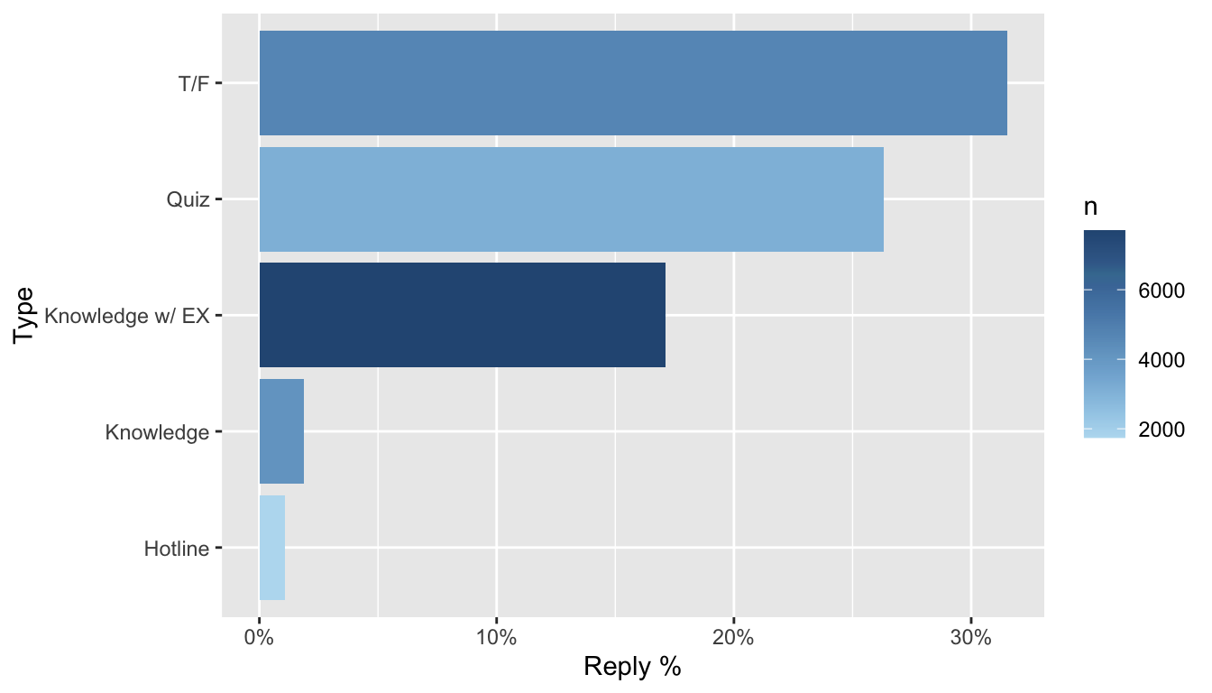
Graph of response rate to each question type
Here’s just an overview of the crude percent of people who responded to each question type:
| Type | Yes | No | Reply % | n |
|---|---|---|---|---|
| Hotline | 19 | 1725 | 1.09% | 1744 |
| Knowledge | 78 | 4082 | 1.87% | 4160 |
| Knowledge w/ EX | 1318 | 6387 | 17.11% | 7705 |
| Quiz | 818 | 2290 | 26.32% | 3108 |
| T/F | 1482 | 3222 | 31.51% | 4704 |
Chi-Squared
TODO: Effect size..?
Contengency table
Contengency table of responded (yes, no) vs the type of question
| Hotline | Knowledge | Knowledge w/ EX | Quiz | T/F | |
|---|---|---|---|---|---|
| Yes | 19 | 78 | 1318 | 818 | 1482 |
| No | 1725 | 4082 | 6387 | 2290 | 3222 |
Test Results
Here’s the test results
chisq.test(conTable)
##
##  Pearson's Chi-squared test
##
## data:  conTable
## X-squared = 1848.9, df = 4, p-value < 2.2e-16
chisq.test(conTable, simulate.p.value = TRUE, B = 10000)
##
##  Pearson's Chi-squared test with simulated p-value (based on 10000
##  replicates)
##
## data:  conTable
## X-squared = 1848.9, df = NA, p-value = 9.999e-05
Residuals
| Hotline | Knowledge | Knowledge w/ EX | Quiz | T/F | |
|---|---|---|---|---|---|
| Yes | -16.30 | -23.96 | -0.50 | 12.02 | 23.32 |
| No | 7.47 | 10.97 | 0.23 | -5.50 | -10.68 |
Post-hoc analysis
Using Fisher’s Exact. Agrees nicely with the results from the logistic regression (next section)
update No longer working because fifer package removed
Binomial
Note: These regressions are run on students who responded at least once
Some resources for binomal regression (for my reference):
Logit model
Run a bimodal regression based on Question type + grade + race + gender
+ number of user's responses + Campaign number (e.g. is it the first message
sent, second sent, last message sent in the campaign).
In the future, can look at how category and/or keywords play into this.
The next table (Table 6) shows the model in a more pretty table format. Table 7 shows the same model, but with an output more similar to SPSS.
| Estimate | Std. Error | z value | Pr(>|z|) | |
|---|---|---|---|---|
| (Intercept) | -6.354 | 0.3701 | -17.17 | 4.606e-66 |
| TypeKnowledge | 0.3154 | 0.3071 | 1.027 | 0.3044 |
| TypeKnowledge w/ EX | 3.931 | 0.2709 | 14.51 | 1.009e-47 |
| TypeQuiz | 4.912 | 0.2784 | 17.64 | 1.197e-69 |
| TypeT/F | 5.029 | 0.2737 | 18.38 | 2.05e-75 |
| grade11 | -0.09469 | 0.08896 | -1.064 | 0.2871 |
| grade12 | -0.0538 | 0.08536 | -0.6303 | 0.5285 |
| grade7 | 0.07815 | 0.1302 | 0.6004 | 0.5482 |
| grade8 | 0.03561 | 0.1804 | 0.1974 | 0.8435 |
| grade9 | -0.095 | 0.0932 | -1.019 | 0.3081 |
| raceAsian | 0.1379 | 0.2794 | 0.4937 | 0.6215 |
| raceBlack | 0.2564 | 0.2511 | 1.021 | 0.3072 |
| raceHispanic | 0.1618 | 0.2426 | 0.6667 | 0.505 |
| raceOther | 0.2364 | 0.2966 | 0.797 | 0.4254 |
| raceWhite | 0.1511 | 0.2419 | 0.6248 | 0.5321 |
| genderMale | -0.008795 | 0.06531 | -0.1347 | 0.8929 |
| genderOther | -0.1408 | 0.3921 | -0.3591 | 0.7195 |
| userResponses | 0.1489 | 0.003566 | 41.76 | 0 |
| campg.num | -0.03787 | 0.002095 | -18.08 | 4.631e-73 |
| Estimate | Std. Error | z value | Pr(>|z|) | |
|---|---|---|---|---|
| (Intercept) | -6.354 | 0.3701 | -17.17 | 0 |
| TypeKnowledge | 0.3154 | 0.3071 | 1.027 | 0.3044 |
| TypeKnowledge w/ EX | 3.931 | 0.2709 | 14.51 | 0 |
| TypeQuiz | 4.912 | 0.2784 | 17.64 | 0 |
| TypeT/F | 5.029 | 0.2737 | 18.38 | 0 |
| grade11 | -0.0947 | 0.089 | -1.065 | 0.2871 |
| grade12 | -0.0538 | 0.0854 | -0.6303 | 0.5285 |
| grade7 | 0.0782 | 0.1302 | 0.6004 | 0.5482 |
| grade8 | 0.0356 | 0.1804 | 0.1974 | 0.8435 |
| grade9 | -0.095 | 0.0932 | -1.019 | 0.3081 |
| raceAsian | 0.1379 | 0.2794 | 0.4937 | 0.6215 |
| raceBlack | 0.2564 | 0.2511 | 1.021 | 0.3072 |
| raceHispanic | 0.1618 | 0.2426 | 0.6667 | 0.505 |
| raceOther | 0.2364 | 0.2966 | 0.797 | 0.4254 |
| raceWhite | 0.1511 | 0.2419 | 0.6248 | 0.5321 |
| genderMale | -0.0088 | 0.0653 | -0.1347 | 0.8929 |
| genderOther | -0.1408 | 0.3921 | -0.3591 | 0.7195 |
| userResponses | 0.1489 | 0.0036 | 41.76 | 0 |
| campg.num | -0.0379 | 0.0021 | -18.08 | 0 |
| Exp(Estimate) | Exp(B) Lower95CI | Exp(B) Upper95CI | |
|---|---|---|---|
| (Intercept) | 0.0017 | 8e-04 | 0.0035 |
| TypeKnowledge | 1.371 | 0.7659 | 2.572 |
| TypeKnowledge w/ EX | 50.95 | 30.93 | 90.02 |
| TypeQuiz | 135.9 | 81.14 | 243.2 |
| TypeT/F | 152.7 | 92.17 | 271.1 |
| grade11 | 0.9097 | 0.7641 | 1.083 |
| grade12 | 0.9476 | 0.8017 | 1.12 |
| grade7 | 1.081 | 0.8364 | 1.393 |
| grade8 | 1.036 | 0.7232 | 1.468 |
| grade9 | 0.9094 | 0.7574 | 1.091 |
| raceAsian | 1.148 | 0.6644 | 1.988 |
| raceBlack | 1.292 | 0.7918 | 2.121 |
| raceHispanic | 1.176 | 0.7322 | 1.897 |
| raceOther | 1.267 | 0.7072 | 2.264 |
| raceWhite | 1.163 | 0.7257 | 1.875 |
| genderMale | 0.9912 | 0.8718 | 1.126 |
| genderOther | 0.8687 | 0.3736 | 1.771 |
| userResponses | 1.161 | 1.153 | 1.169 |
| campg.num | 0.9628 | 0.9589 | 0.9668 |
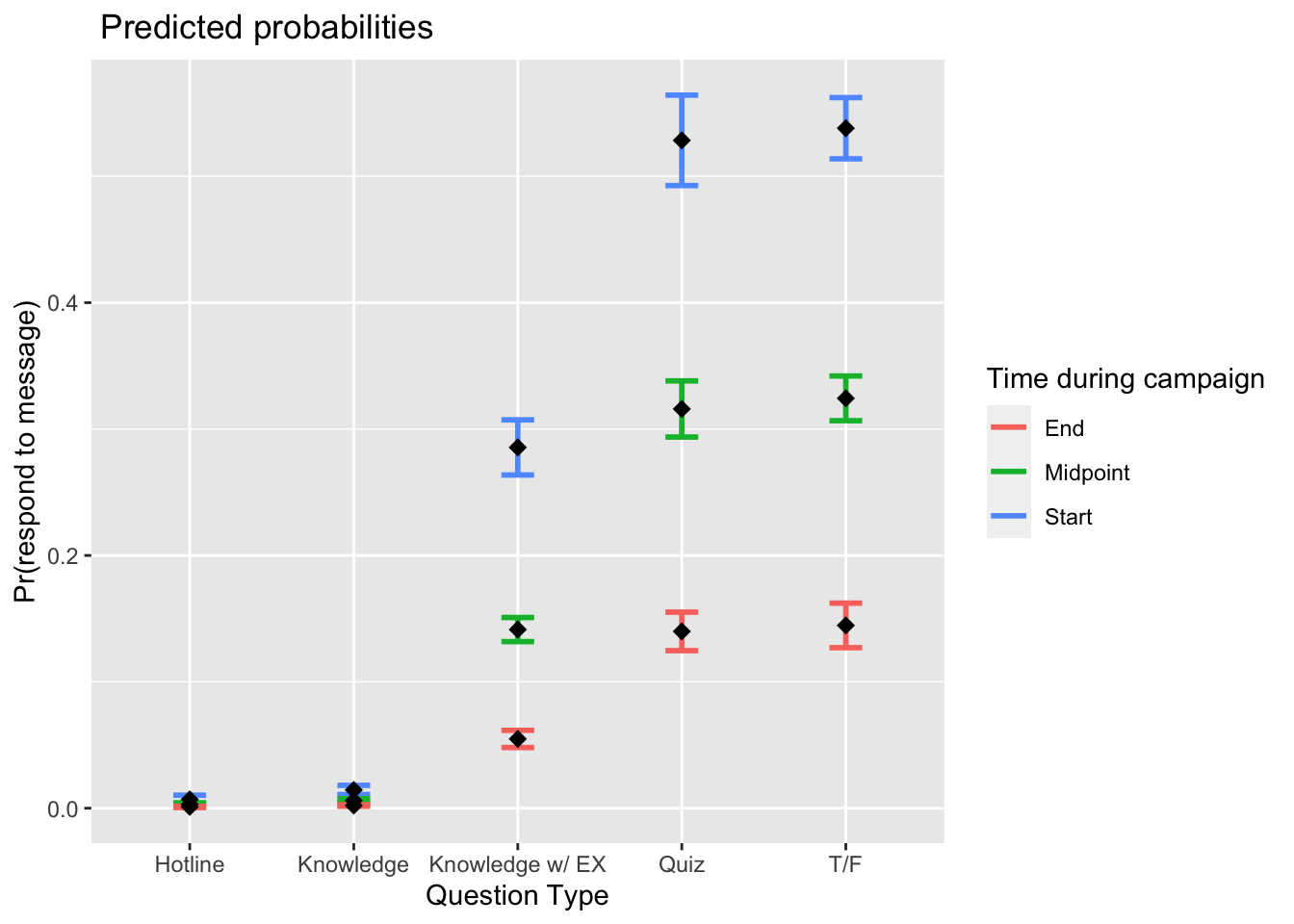
Prediction
Based on modeling only the significant variables from above, which has a higher
AIC (second model’s AIC=12,331) than the model above (AIC=8,090). Note that
the figure shows three points in time (beginning, midpoint, and end), but assumes
userResponses is the same across the board
Multilevel logit model
The next output below models the fixed effects of variables of interest
(e.g. question type) while accounting for random effects (userID). Note:
the model doesn’t converge if gender, race, or grade is included, presumably
because those effects are accounted for in the random effects of the userID
## Generalized linear mixed model fit by maximum likelihood (Laplace
## Approximation) [glmerMod]
## Family: binomial ( logit )
## Formula: Replied ~ Type + (1 | userID)
## Data: df
##
## AIC BIC logLik deviance df.resid
## 12952.6 12999.4 -6470.3 12940.6 18068
##
## Scaled residuals:
## Min 1Q Median 3Q Max
## -4.1588 -0.3957 -0.1975 -0.0403 24.7967
##
## Random effects:
## Groups Name Variance Std.Dev.
## userID (Intercept) 2.119 1.456
## Number of obs: 18074, groups: userID, 414
##
## Fixed effects:
## Estimate Std. Error z value Pr(>|z|)
## (Intercept) -5.3448 0.2489 -21.474 <2e-16 ***
## TypeKnowledge 0.5810 0.2626 2.212 0.0269 *
## TypeKnowledge w/ EX 3.4863 0.2392 14.572 <2e-16 ***
## TypeQuiz 4.2730 0.2426 17.613 <2e-16 ***
## TypeT/F 4.7069 0.2411 19.524 <2e-16 ***
## ---
## Signif. codes: 0 '***' 0.001 '**' 0.01 '*' 0.05 '.' 0.1 ' ' 1
##
## Correlation of Fixed Effects:
## (Intr) TypKnw TKw/EX TypeQz
## TypeKnowldg -0.842
## TypKnwlw/EX -0.942 0.876
## TypeQuiz -0.934 0.864 0.967
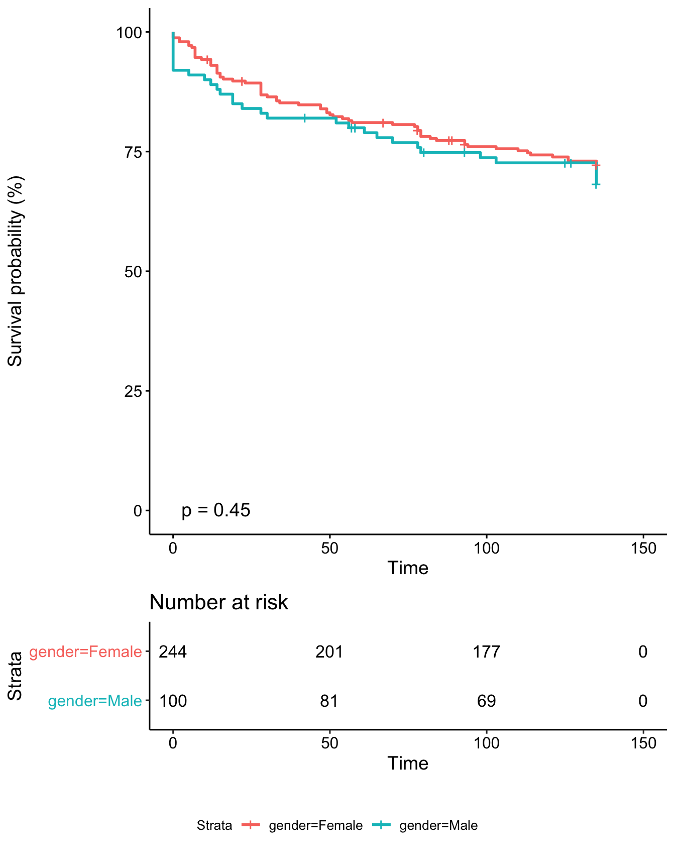
## TypeT/F -0.943 0.870 0.974 0.966Survival analysis
Some resources for survival analysis (for my reference):
Gender
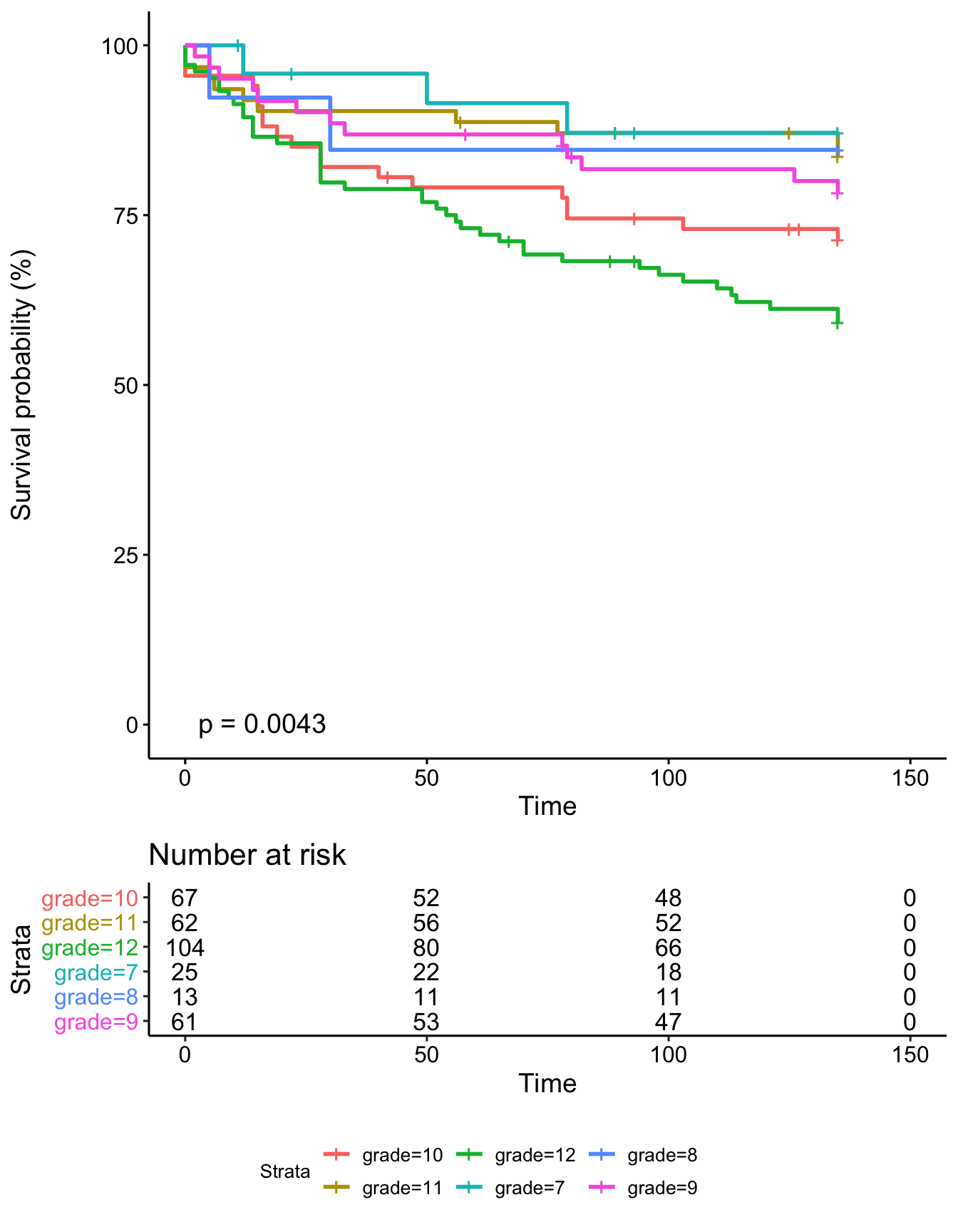
Grade
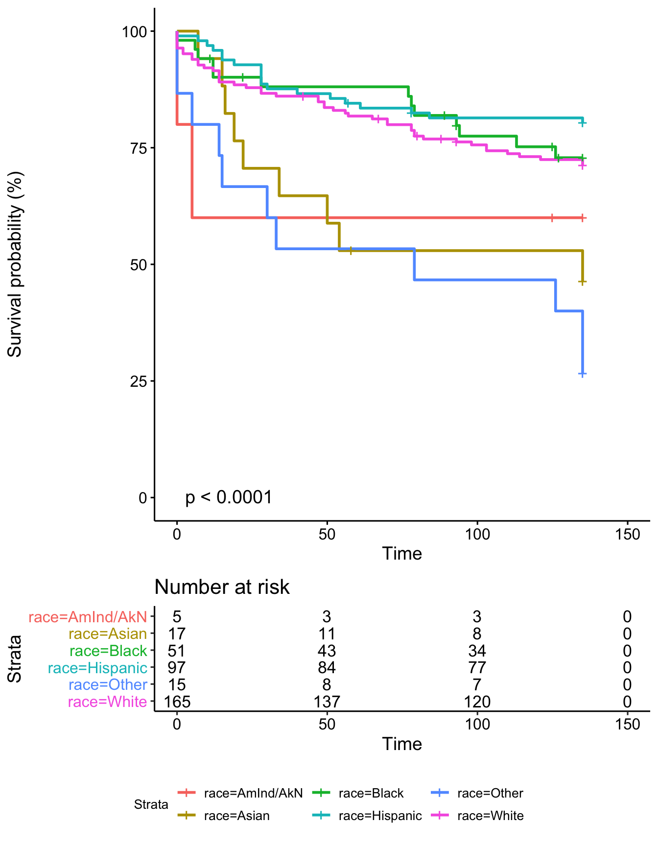
Race
Combo
Descriptive statistics
So there’s quite a few NA’s (people who didn’t have their gender, grade, or race
recorded). A few people did respond to the gender & grade questions, but didn’t
fit into a larger category, so I dropped them from the analysis (total of 7 students)
Total number of students: 525
Gender
| gender | n | sansNA | Percent |
|---|---|---|---|
| Female | 238 | 72% | 45.9% |
| NA | 189 | 0% | 36.4% |
| Male | 92 | 28% | 17.7% |
Grade
| grade | n | sansNA | Percent |
|---|---|---|---|
| NA | 207 | 0% | 40% |
| 12 | 99 | 31% | 19% |
| 10 | 64 | 20% | 12% |
| 11 | 58 | 18% | 11% |
| 9 | 58 | 18% | 11% |
| 7 | 25 | 8% | 5% |
| 8 | 13 | 4% | 2% |
Race
Note that unlike gender & grade, I didn’t drop the Other race because it’s
representing Two or more races
| race | n | sansNA | Percent |
|---|---|---|---|
| NA | 189 | 0.0% | 36.00% |
| White | 157 | 46.7% | 29.90% |
| Hispanic | 96 | 28.6% | 18.29% |
| Black | 50 | 14.9% | 9.52% |
| Asian | 17 | 5.1% | 3.24% |
| Other | 12 | 3.6% | 2.29% |
| AmInd/AkN | 4 | 1.2% | 0.76% |
Compare to Census data (2017 ACS 5-year estimates) from Galveston County:
| Race | Percent |
|---|---|
| White (non-Hispanic) | 45.90% |
| Hispanic or Latino | 28.70% |
| Black or African American | 20.80% |
| Asian | 3.20% |
| Two or more races | 2.50% |
| American Indian and Alaska Native | 0.50% |
Session info
R version 3.6.3 (2020-02-29)
Platform: x86_64-apple-darwin15.6.0 (64-bit)
locale: en_US.UTF-8||en_US.UTF-8||en_US.UTF-8||C||en_US.UTF-8||en_US.UTF-8
attached base packages: stats, graphics, grDevices, utils, datasets, methods and base
other attached packages: pander(v.0.6.3), survMisc(v.0.5.5), survminer(v.0.4.6), ggpubr(v.0.2.5), magrittr(v.1.5), survival(v.3.1-8), lme4(v.1.1-21), Matrix(v.1.2-18), stargazer(v.5.2.2), scales(v.1.1.0), knitr(v.1.28), lubridate(v.1.7.4), forcats(v.0.5.0), stringr(v.1.4.0), dplyr(v.0.8.5), purrr(v.0.3.4), readr(v.1.3.1), tidyr(v.1.1.0), tibble(v.3.0.0), ggplot2(v.3.3.0), tidyverse(v.1.3.0) and MASS(v.7.3-51.5)
loaded via a namespace (and not attached): httr(v.1.4.1), jsonlite(v.1.6.1), splines(v.3.6.3), modelr(v.0.1.6), assertthat(v.0.2.1), highr(v.0.8), cellranger(v.1.1.0), yaml(v.2.2.1), pillar(v.1.4.3), backports(v.1.1.6), lattice(v.0.20-38), glue(v.1.4.0), digest(v.0.6.25), ggsignif(v.0.6.0), rvest(v.0.3.5), minqa(v.1.2.4), colorspace(v.1.4-1), htmltools(v.0.4.0), pkgconfig(v.2.0.3), broom(v.0.5.5), haven(v.2.2.0), bookdown(v.0.18), xtable(v.1.8-4), km.ci(v.0.5-2), KMsurv(v.0.1-5), farver(v.2.0.3), generics(v.0.0.2), ellipsis(v.0.3.0), withr(v.2.1.2), cli(v.2.0.2), crayon(v.1.3.4), readxl(v.1.3.1), evaluate(v.0.14), fs(v.1.4.1), fansi(v.0.4.1), nlme(v.3.1-144), xml2(v.1.3.0), ggthemes(v.4.2.0), blogdown(v.0.18), data.table(v.1.12.8), tools(v.3.6.3), hms(v.0.5.3), lifecycle(v.0.2.0), munsell(v.0.5.0), reprex(v.0.3.0), compiler(v.3.6.3), rlang(v.0.4.6), grid(v.3.6.3), nloptr(v.1.2.2.1), rstudioapi(v.0.11), labeling(v.0.3), rmarkdown(v.2.1), boot(v.1.3-24), gtable(v.0.3.0), DBI(v.1.1.0), R6(v.2.4.1), zoo(v.1.8-7), gridExtra(v.2.3), stringi(v.1.4.6), Rcpp(v.1.0.4.6), vctrs(v.0.3.0), dbplyr(v.1.4.2), tidyselect(v.1.1.0) and xfun(v.0.13)
Hunter Ratliff, MD, MPH
Infectious Diseases Fellow
My research interests include epidemiology, social determinants of health, and reproducible research.